Chapter 7

The only relevant test of the validity of a hypothesis is comparison of its predictions with experience.
Milton Friedman (1912 - 2006) Economist and Statistician

Humor Alert: I don't know why people are so negative about statistics and statisticians. I'm only a first-year student, and statistics has already taught me everything I need to know about life - always Proceed with Caution and Reject H₀! - Priscilla Mok

The Runs Test addresses only nominal data, only two data categories, and only whether or not the sample observed was drawn from a population that is generated randomly. An examination of runs can assist in deciding upon the randomness or nonrandomness of what is actually observed. Runs can be used to formulate tests of hypotheses regarding the randomness of the population from which the sample was drawn.

H₀: the number of runs observed is due to chance, that nothing is influencing the generation of runs, H₀: number of runs = what is expected from a chance or random process
H₁: the number of runs observed is due to some factor other than chance, that something is influencing the generation of runs, H₁: number of runs ≠ what is expected from a chance or random process

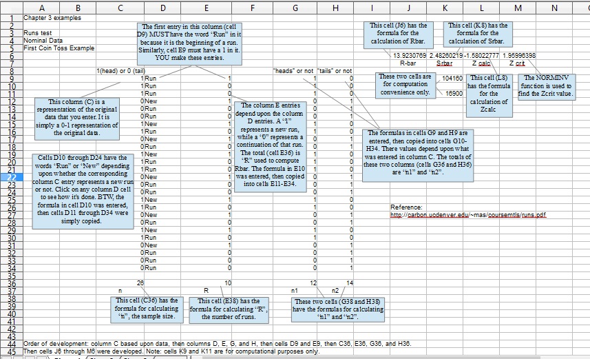
A run is defined as a simply a series (1 or more) of two differing values. For example, consider tossing a coin 26 times (the sample size: n=26) with this result:

In the example above, there are 10 runs (each run is underlined), which is the observed number of runs. Note that a run can be of any length: from 1 to ∞.

are calculated. That is all that is needed. Using these formulae, the expected number of runs (R_bar), and the variance of the expected number of runs (S²_Rbar) can be calculated.

Expected number of runs = R_bar = (2* n₁* n₂)/(( n₁+ n₂)+1)
where: n₁ is the number of "1"s ("H") observed, and n₂ is the number of "0"s ("T") observed

The variance of the Expected number of runs S_Rbar = ((2*n₁*n₂)*(2*n₁*n₂-n₁-n₂))/(( n₁* n₂)²)+(n₁+n₂-1)) The standard deviation (needed to calculate Z_calc) is simply the square root of the variance.

The above formulae appears formidable, so thank goodness for the "COPY" command, and that the RUNS spreadsheets can be downloaded. In other words, the hard work has already been done for you!

So, the test statistic, conveniently named Z, is (the absolute value of): (observed number of runs - R_bar)/ √ (σ²), and is called Z_calc.
Also, Z_calc = [(observed number of runs - R_bar)/σ] Note: this is the way it is calculated in the spreadsheets.

The test statistic is approximately normally distributed, so you can make good decisions by using the OpenOffice Normal Distribution function NORMINV.

WARNING: in order to use the OpenOffice NORMINV function properly, the value of α (typically 0.05) MUST be halved, then subtracted from 1. That value (typically 0.975) is entered as the first argument into the NORMINV function(1 - α/2). The second and third arguments are ALWAYS 0 and 1 (the mean and standard deviation of the normal probability distribution are 0 and 1).

You can, alternately, use the NORMSINV function, where the second and third arguments (0 and 1) are assumed. All else is the same. Both functions return the same value.

Here is how you find the appropriate value by using the NORMINV function to get the "critical" Z value.
Typically, α = .05 (you want to be [at least] 95% confident that you are correct regarding your decision about H₀), so first divide α by 2, yielding .025.
    Subtract that from 1, yielding .9750, the first argument value entered in the NORMINV function (the second and third arguments are ALWAYS 0 and 1). The value returned is 1.95996... (or 1.96). This is your "critical" Z value.
    Use this procedure to find the "critical" Z value when conducting any test (in this book) when using the NORMINV function.
    The reason you must use this procedure is because the NORMINV function is not suitable for direct use (because the OpenOffice programmers said so!)

Now calculate the test statistic (Z_calc) using the formula above: how many standard deviations what was actually observed (in your sample) is from the expected (hypothesized) number of runs (R_Bar). This quantity is called your calculated Z score or value. Why Z? Why not? It has to be called something. Z_calc, your calculated Z score, is actually the number of standard deviations what you observed differs from what you expected (hypothesized).

Now compare your calculated Z score with the Z returned by NORNINV (often called the critical Z - note that "critical" is just a communication convenience).
IF your calculated Z score is greater than the "critical" Z, REJECT H₀ and make your managerial decision based upon some other criterion (usually what you observed since it is available and you have nothing else upon which to go).

IF your calculated Z score is NOT greater than the "critical" Z, fail to reject H₀ (which is NOT the same as accepting H₀) and make your managerial decision as if H₀ is correct. (Note that H₀ was not accepted, or proven correct, or proven to be true, just not rejected.)

NOTE: if H₀ is correct (something you will never know for certain), then Z_calc will be "close" to zero. So, comparing Z_calc to Z_crit is the "statistics" way of comparing what you observed from the sample to what you hypothesized.

In the coin toss example above, there are 10 runs (observed), the expected number of runs (R_bar) is 13.923, the standard deviation (square root of variance) of the expected number of runs (√S_Rbar) is 2.482, so the Z_calc score is -1.580
or Z_calc = (10-13.923/2.482)
or Z_calc = -1.580

The minus sign (-) indicates only that the number of runs observed is less than the number expected. So compare the absolute value of your calculated Z (1.580) score against your "critical" Z (1.95996). In this example, 1.580 is not greater than 1.95996 (the "critical" Z value returned by NORMINV), so DO NOT reject H₀. Your managerial decision can now be based what you observed as having been produced randomly since you could not, based on sample evidence, reject the idea of random production.

You are (at least) 95% confident that you are making the correct decision regarding H₀, which states that the coin toss runs pattern observed was generate by a random process.

Notice that the Runs Test did NOT make the decision whether H₀ should be rejected or not. It only provided information so that the decision maker (you) can make a decision.

Below is the spreadsheet used to conduct the "Runs" test. This spreadsheet is part of "ch7-ex.xls" which can be downloaded for further inspection, as well as for copying.

Notice that R_bar, S_Rbar, and Z_calc are all part of the spreadsheet that can be downloaded. You can copy these formulae, then modify them to be used with your sample. The "hard work" has already been done for you. This is true for ALL nonparametric procedures presented in this book.

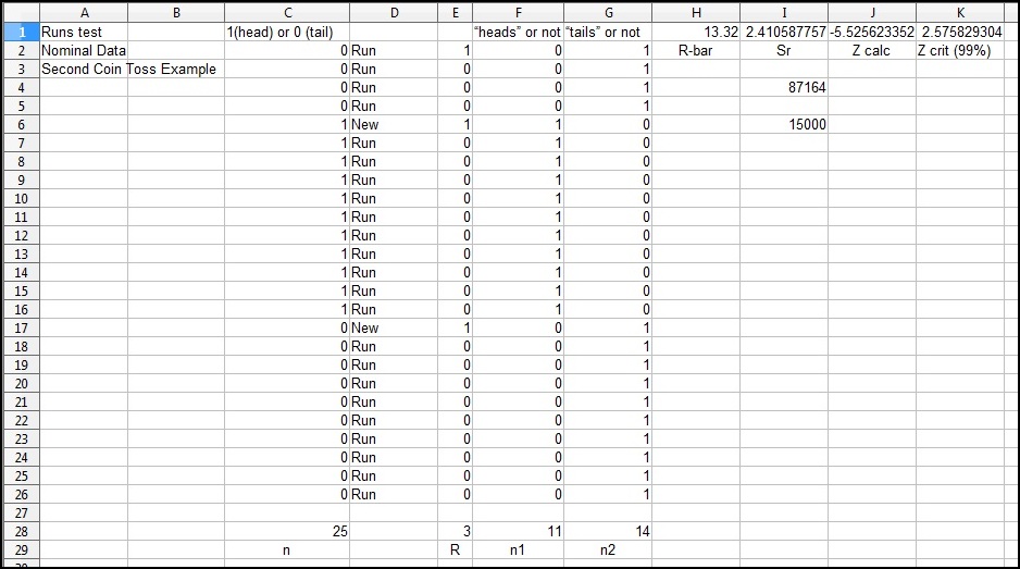
Consider again the tossing of a coin. Let's say you toss the coin 25 times, with this result:

You want to be (at least) 99% certain that you are correct when making a decision about the randomness of the coin toss process.

H₀: The coin toss process is random, that the pattern observed was generated by a random process
H₁: Not H₀, The coin toss process is NOT random, that the pattern observed was NOT generated by a random process
That is step 1.

α = 0.01 (you want to be 99% certain that you are making the correct decision, so α is .01)

To use the NORMINV function, you first divide α by 2, subtract that value from 1, then enter that value. The "critical" value of Z is returned. It is that simple!
In this example, the critical Z value is determined by:
1 - α/2 = .995, so .995 is entered into the NORMINV function.

Now it is time to take your sample (toss the coin and observe the number of runs - the data above), then calculate how much what you observed differs from H₀ (what you expect) in sample standard deviations. The "sample" is in the spreadsheet.

Now compare (the absolute value of) your calculated Z score (-5.526) with your critical Z score (2.57).

From this sample evidence, you can determine that the pattern (number of runs) was not generated by a random process, that the coin toss process is not random (you rejected the idea that it was). You are (at least) 99% confident that you are correct when describing the coin toss process. (Note: you did not prove H₁ to be true)

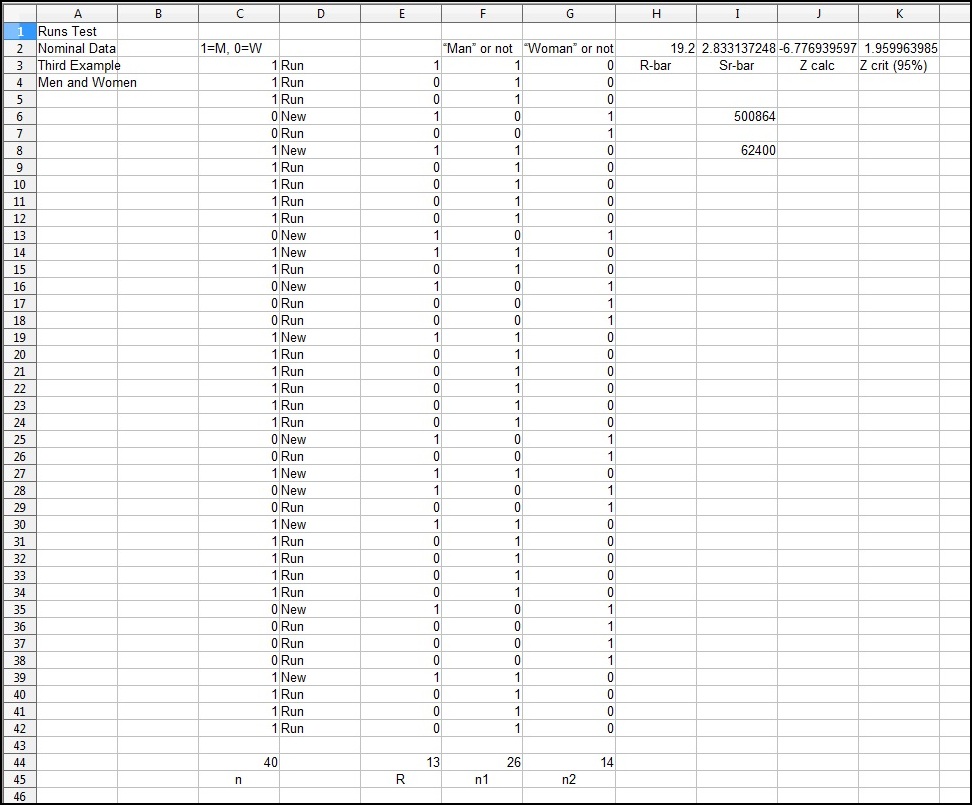
Let's assume that you own a "sports bar," and that you have spent quite a large sum of money on advertising to attract women to the bar. Now you want to see if the money spent on advertising was effective. You randomly select several nights, several different hours from the nights, then observe the men and women as they enter the bar:

H₀: pattern (Runs) observed is random, sample was drawn from a random population (advertising was not effective)
H₁: pattern (Runs) observed is not random, sample was not drawn from a random population (advertising was effective)

You want to be (at least) 95% certain that you are making the correct decision regarding H₀ (advertising NOT effective), so Z_crit = 1.9599.

In this example, N = 40, R_bar = 19.2, S² = 8.00, so S = 2.83, n1 = 26, n2 = 14, Z_calc = -6.77, and Z_crit = 1.9599.

You CAN, based upon your hypothesis test, reject H₀. You are inclined, based on the sample observed, to conclude (but did not prove) that the advertising is effective, and make your managerial decision accordingly. Note that you did not PROVE H₁ to be correct, only that you rejected H₀.

The Sign Test is used in a one population situation to determine whether a population median (usually opinions) is equal to or not equal to a specific hypothesized number. It makes very few assumptions about the nature of the distribution of the population being examined, so it has very general applicability. The sign test allocates a sign, either positive (+) or negative (-), to each observation according to whether it is greater or less than some hypothesized value (usually the hypothesized median value), and considers whether the pattern of "+"s and "-"s is substantially different from what we would expect by chance.

Any sample of size of less than 25 is considered to be small, and the table in the appendix can be used to determine the "critical" sign test value.

For a sample size of 25 or greater, the results of the Sign Test closely approximate the Normal probability distribution, so NORMINV can be used.

Suppose that you are the manager of a fast food restaurant, and want to see whether your opinion that the median satisfaction score of customers who try (for free) a new product is correct or not. You think the median satisfaction score is 90. You want to be (at least) 95% confident that you are correct regarding your decision about H₀, so α=0.05. You randomly select 12 people, have them try the new product, then offer a satisfaction score. The spreadsheet illustration below shows the scores and procedure:

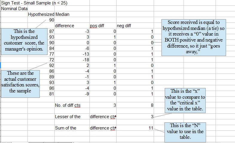
The lesser of the differences totals (4) is NOT less than the "critical" value of 2 (α=.05, N=12) found in the table, so H₀ CANNOT be rejected. There is not enough observed evidence to cause you to abandon your opinion that the satisfaction score median is 90.

Observed values equal to the hypothesized median, the ties, receive a 0 value for both differences, so they "go away."

For large sample (n =>25), the calculated Sign Test value, Z_calc, is approximately normally distributed, so the NORMINV function can be used.

The formula for Z_calc is: ( (X + 0.5 ) - (N - 2) ) / ( SQRT(N) / 2 )
where X and N are calculated by the Sign Test procedure: X= lesser of + or - count; N = sum of + and - counts, ties ignored.
Again, this formula appears formidable. But don't worry, it can be copied.

If the (absolute value of the) calculated Z score is greater than the "critical" Z score returned by NORMINV, reject H₀. Otherwise, fail to reject H₀.

Note that "n" is the sample size, while "N" is the sum of + and - counts, ties ignored.

Say that as a manager of a large company, you think that your employees have a median score of 35 on some arbitrary classification score that does not connote any ranking. You randomly select 30 employees, classify them, and record the scores. You want to be (at least) 95% confident that you are correct regarding your decision about H₀, so α=0.05, and the NORNSINV function is used to get Z_crit (so α/2 is entered into the function). The spreadsheet illustrations below shows the scores and procedure:

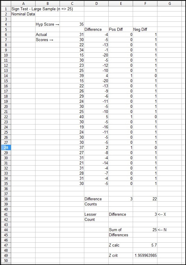
As can be seen, Z_calc is greater than Z_crit, so H₀ CAN be rejected (note: you did not prove H₁ to be true) and you can be (at least) 95% confident that you are correct when you say the median classification score is NOT 35. What is the median classification score? The Sign Test cannot answer that question.

The Wilcoxon Signed Rank Test is used to make an inference about the median of one population. The procedure requires the specification of (what is thought to be) the median of the population of interest.

Let's assume that you are the manager of a large company, and that you have ranked employees with respect to their effectiveness when dealing with potential customers, with higher rank scores indicating that they are more effective. Now you want to see if the median rank score assigned is 4. This is your null hypothesis: H₀ median score = 4. Alternately, the median rank score may not be 4: H₁ median score ≠ 4.

You randomly select nine (n = 9) employees, record their scores, and analyze the scores. The analysis is illustrated below:

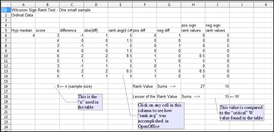
The "rule" is that if the "W" value from the analysis is not less than the "critical W" value from the table, DO NOT reject H₀. If the "W" value from the analysis is LESS than the "critical W" value from the table, reject H₀.

The calculated "W" value is 15. This is the value compared to the "critical W" value from the appendix table, which (for n=9, α=.05) is 5. Since the calculated "W" value of 15 is larger than (not less than) the "critical W" value of 5, do NOT reject H₀. There is no compelling evidence, based on the sample, that the median score ≠ 4. Make the managerial decision accordingly.

Two notes are in order here: (1) Samples of size 20 or smaller MUST use the procedure illustrated above and the table in the appendix. Sample sizes less than 5 cannot be analyzed. Sample sizes greater than 20 can use either the table (if applicable) or the normal approximation method (below); (2) "W" is approximately normally distributed for samples of size greater than 20, so the NORMINV function can be used.

The situation described in the above example has, in this example, been expanded to 25 people's scores (n = 25) so that a large sample is created. The function NORMINV can be used for a normal approximation, as can the table. The spreadsheet is illustrated below:

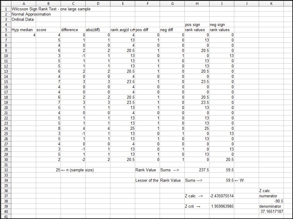
For a sample size of 25, a "W" value of 59.5 is calculated. From the table (α = .05), the "critical" W value is 89, so, the H₀ CAN be rejected.

As can be seen in the spreadsheet, the (absolute value of) Z_calc value of -2.435 is greater than the Z_crit value of 1.959 returned by NORMINV. So, the H₀ CAN be rejected.

You CANNOT validly play "what if" by entering different median score values until H₀ cannot be rejected because analyzing the same sample numerous times inflates the probability of committing a Type I error.

NOTE: The Wilcoxon Signed Rank Test table goes as high as "n = 30, but following these rules will "keep you out of trouble."

You have been introduced to one population hypothesis testing using the RUNS Test, the SIGN Test, and the WILCOXON SIGN RANK Test.

One Population